News and Enhancements of rpact, an R Package for Adaptive Confirmatory Designs

Kolloquium Statistische Methoden in der empirischen Forschung

Gernot Wassmer, Friedrich Pahlke, Daniel Sabanés Bové

RPACT GmbH

January 13, 2026

Seven Years Ago

The rpact Package 📦

• Comprehensive validated R package implementing methodology described in Wassmer and Brannath (2016)
• Enables the design of traditional and confirmatory adaptive group sequential designs
• Provides interim data analysis and simulation including early efficacy stopping and futility analyses
• Enables sample-size reassessment with different strategies
• Enables treatment arm selection in multi-stage multi-arm (MAMS) designs
• Enables subset selection in population enrichment designs
• Provides a comprehensive and reliable sample size calculator

Developed by RPACT 🏢

• RPACT GbR company founded in 2017 by Gernot Wassmer and Friedrich Pahlke
• Idea: open source development with help of “crowd funding”
• Currently supported by 21 companies
• \(>\) 80 presentations and training courses since 2018, e.g., FDA in March 2022
• 30 vignettes based on Quarto and published on rpact.org/vignettes
• 28 releases on CRAN since 2018

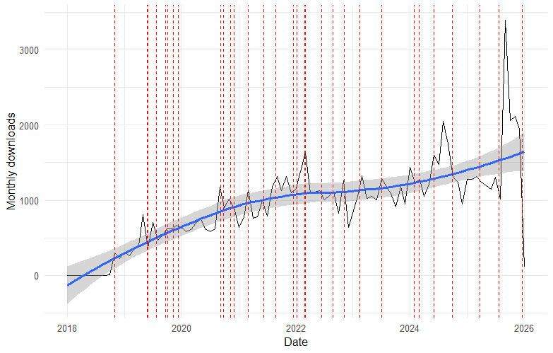
CRAN Downloads ✌️

RCONIS 🚀

• Grow RPACT company to offer a wider range of services
• Statistical consulting and engineering services: Research Consulting and Innovative Solutions
• Joint venture between RPACT GmbH (rpact.com) and inferential.biostatistics GmbH (inferential.bio) founded by Daniel Sabanés Bové and Carrie Li
• Website: rconis.com

Second Edition of the Book

• Provides up-to-date overview of group sequential and confirmatory adaptive designs in clinical trials
• Describes available software including R packages and has rpact code examples
• Supplemented with a discussion of practical applications
• Published Oct 2025

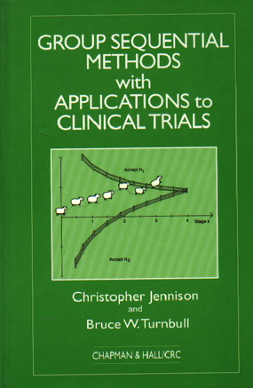
Second Edition of Jennison and Turnbull

Jennison and Turnbull, 1999

Published Dec 2025

The R Package rpact – Functional Range

Trial Designs 🔬

• Fixed sample designs:
  • continuous, binary, count, survival outcomes
• Group sequential designs:
  • efficacy interim analyses, futility stopping, alpha-spending functions
• Adaptive designs:
  • Inverse normal and Fisher’s combination test, conditional error rate principle
  • Provides adjusted confidence intervals and bias corrected estimates
  • Multi-arm multi-stage (MAMS) and enrichment designs, sample size reassessment

Easy to understand R commands:

getDesignGroupSequential()
getDesignInverseNormal()
getDesignFisher()
getDesignConditionalDunnett()

Sample Size and Power Calculation 💻

Sample size and power can be calulcated for testing:

• means (continuous endpoint)
• proportions (binary endpoint)
• hazards (survival endpoint)
  • Note: flexible recruitment and survival time options
• rates (count endpoint)

Easy to understand R commands:

getSampleSize[Means / Rates / Survival / Counts]()
getPower[Means / Rates / Survival / Counts]()

Example: Sample Size Calculation 🧮

# Define the design.
getDesignGroupSequential(
    typeOfDesign = "asOF",
    futilityBounds = c(0, 0)
) |>
    # Perform sample size calculation.
    getSampleSizeMeans(
        alternative = 2,
        stDev = 5
    ) |>
    # Obtain summary.
    summary()

Sample size calculation for a continuous endpoint

Sequential analysis with a maximum of 3 looks (group sequential design), one-sided overall significance level 2.5%, power 80%. The results were calculated for a two-sample t-test, H0: mu(1) - mu(2) = 0, H1: effect = 2, standard deviation = 5.

Stage	1	2	3
Planned information rate	33.3%	66.7%	100%
Cumulative alpha spent	0.0001	0.0060	0.0250
Stage levels (one-sided)	0.0001	0.0060	0.0231
Efficacy boundary (z-value scale)	3.710	2.511	1.993
Futility boundary (z-value scale)	0	0
Efficacy boundary (t)	4.690	2.152	1.384
Futility boundary (t)	0	0
Cumulative power	0.0204	0.4371	0.8000
Number of subjects	69.9	139.9	209.8
Expected number of subjects under H1			170.9
Overall exit probability (under H0)	0.5001	0.1309
Overall exit probability (under H1)	0.0684	0.4202
Exit probability for efficacy (under H0)	0.0001	0.0059
Exit probability for efficacy (under H1)	0.0204	0.4167
Exit probability for futility (under H0)	0.5000	0.1250
Exit probability for futility (under H1)	0.0480	0.0035

Legend:

• (t): treatment effect scale

Adaptive Analysis 📈

• Perform interim and final analyses during the trial using group sequential method or p-value combination test (inverse normal or Fisher)

• Calculate adjusted point estimates and confidence intervals (cf., Robertson et al. (2023), Robertson et al. (2025))

• Perform sample size reassessment using the observed data, e.g., based on calculation of conditional power

Easy to understand R commands:

getStageResults()
getRepeatedConfidenceIntervals()
getConditionalPower()
getAnalysisResults()

• Some highlights:

  • Automatic boundary recalculations during the trial for analysis with alpha spending approach, including under- and over-running
  • Adaptive analysis tools for multi-arm trials and enrichment designs

Simulation Tool 🧪

Obtain operating characteristics of different designs:

• Assessment of adaptive sample size recalculation strategies
• Assessment of treatment selection strategies in multi-arm trials
• Assessment of population selection strategies in enrichment designs

Easy to understand R commands:

getSimulation[MultiArm / Enrichment][Means / Rates / Survival / Counts]()

Example:

getSimulationMeans()
getSimulationMultiArmMeans()
getSimulationEnrichmentMeans()

Recent Updates

1. Specification of Futility Bounds

Current situation:

getDesignGroupSequential(
  kMax = 3,
  alpha = 0.025,
  sided = 1,
  typeOfDesign = "OF",
  futilityBounds = c(0, -Inf)  
) |> summary()

Sequential analysis with a maximum of 3 looks (group sequential design)

O’Brien & Fleming design, non-binding futility, one-sided overall significance level 2.5%, power 80%, undefined endpoint, inflation factor 1.0628, ASN H1 0.8528, ASN H01 0.8821, ASN H0 0.7059.

Stage	1	2	3
Planned information rate	33.3%	66.7%	100%
Cumulative alpha spent	0.0003	0.0072	0.0250
Stage levels (one-sided)	0.0003	0.0071	0.0225
Efficacy boundary (z-value scale)	3.471	2.454	2.004
Futility boundary (z-value scale)	0	-Inf
Cumulative power	0.0356	0.4617	0.8000
Futility probabilities under H1	0.048	0

Or derivation of futility bounds through beta spending approach

x <- getDesignGroupSequential(
  kMax = 3,
  alpha = 0.025,
  sided = 1,
  typeOfDesign = "asOF",
  typeBetaSpending = "bsKD",
  gammaB = 1.3,
  futilityStops = c(TRUE, FALSE)
) 
summary(x)

Sequential analysis with a maximum of 3 looks (group sequential design)

O’Brien & Fleming type alpha spending design and Kim & DeMets beta spending (gammaB = 1.3), non-binding futility, futility stops c(TRUE, FALSE), one-sided overall significance level 2.5%, power 80%, undefined endpoint, inflation factor 1.0586, ASN H1 0.8634, ASN H01 0.8829, ASN H0 0.7038.

Stage	1	2	3
Planned information rate	33.3%	66.7%	100%
Cumulative alpha spent	0.0001	0.0060	0.0250
Cumulative beta spent	0.0479	0.0479	0.2000
Stage levels (one-sided)	0.0001	0.0060	0.0231
Efficacy boundary (z-value scale)	3.710	2.511	1.993
Futility boundary (z-value scale)	-0.001	-Inf
Cumulative power	0.0204	0.4370	0.8000
Futility probabilities under H1	0.048	0

plot(x)

Fisher’s Combination Test

getDesignFisher(
  kMax = 3,
  alpha = 0.025,
  sided = 1,
  method = "fullAlpha",
  alpha0Vec = c(0.5, 1)
) |> summary()

Sequential analysis with a maximum of 3 looks (Fisher’s combination test design)

Full last stage level design, binding futility, one-sided overall significance level 2.5%, undefined endpoint.

Stage	1	2	3
Fixed weight	1	1	1
Cumulative alpha spent	0.0084	0.0128	0.0250
Stage levels (one-sided)	0.0084	0.0084	0.0250
Efficacy boundary (p product scale)	0.0084123	0.0010734	0.0007284
Futility boundary (separate p-value scale)	0.5000	1.0000

Problem

• For group sequential designs, futility bounds have to be specified on the \(z\)-value scale. For Fisher’s combination test, they are on the separate \(p\)-value scale

• It is desired , however, to define it also for other scales, e.g., the conditional power scale

• On the effect size scale, futility bounds are already the output in the getSampleSize...() and getPower...() function. For example,

getSampleSizeMeans(
  design = 
    getDesignGroupSequential(
      kMax = 3,
      alpha = 0.025,
      sided = 1,
      typeOfDesign = "OF",
      futilityBounds = c(0, 0.5) 
    ),
    alternative = c(0.3, 0.5),
    normalApproximation = TRUE
  ) |> summary()

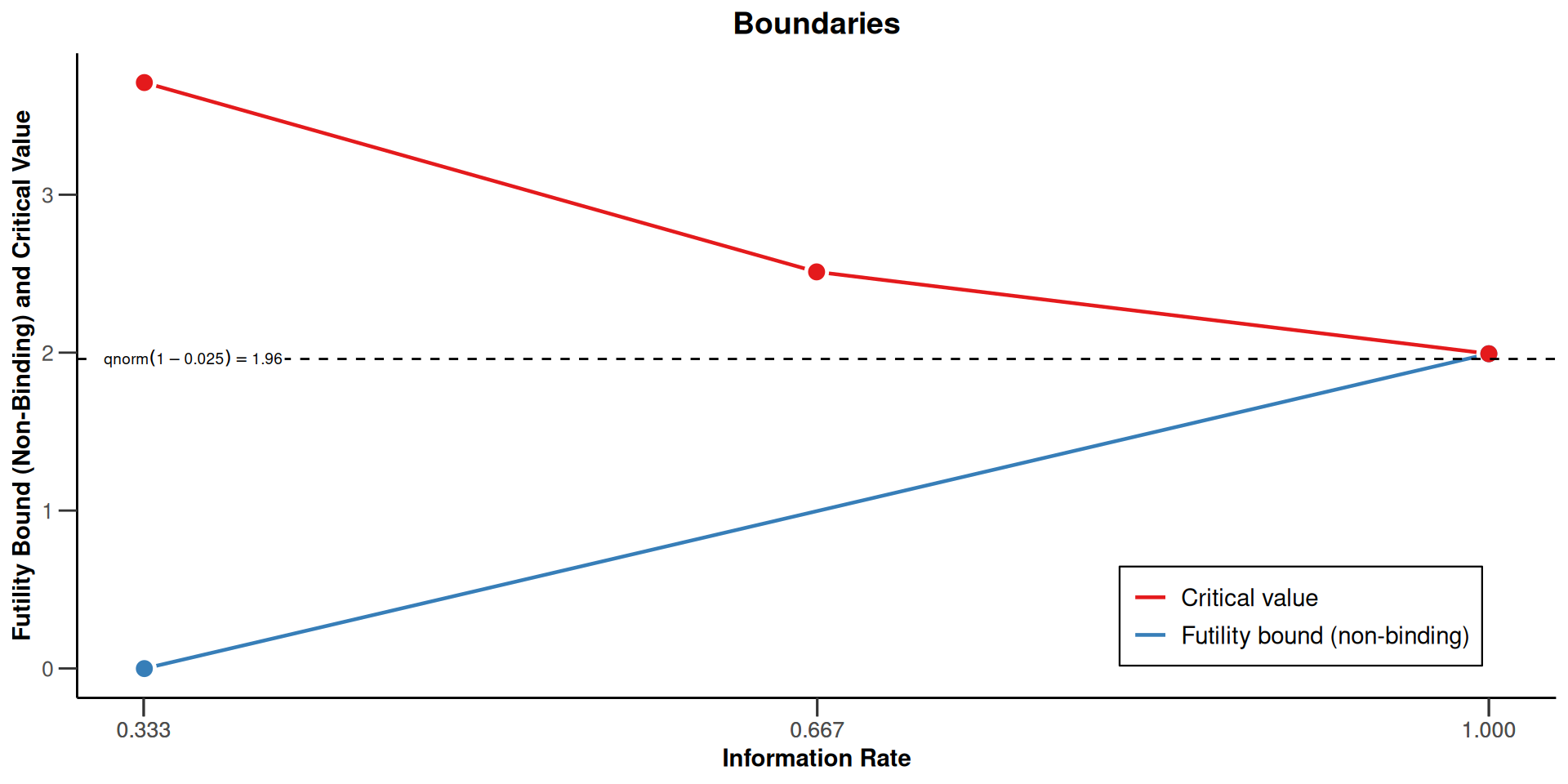
Sample size calculation for a continuous endpoint

Sequential analysis with a maximum of 3 looks (group sequential design), one-sided overall significance level 2.5%, power 80%. The results were calculated for a two-sample t-test (normal approximation), H0: mu(1) - mu(2) = 0, H1: effect as specified, standard deviation = 1.

Stage	1	2	3
Planned information rate	33.3%	66.7%	100%
Cumulative alpha spent	0.0003	0.0072	0.0250
Stage levels (one-sided)	0.0003	0.0071	0.0225
Efficacy boundary (z-value scale)	3.471	2.454	2.004
Futility boundary (z-value scale)	0	0.500
Efficacy boundary (t), alt. = 0.3	0.623	0.312	0.208
Efficacy boundary (t), alt. = 0.5	1.039	0.520	0.346
Futility boundary (t), alt. = 0.3	0	0.064
Futility boundary (t), alt. = 0.5	0	0.106
Cumulative power	0.0359	0.4633	0.8000
Number of subjects, alt. = 0.3	124.0	248.0	372.0
Number of subjects, alt. = 0.5	44.6	89.3	133.9
Expected number of subjects under H1, alt. = 0.3			296.2
Expected number of subjects under H1, alt. = 0.5			106.6
Overall exit probability (under H0)	0.5003	0.2459
Overall exit probability (under H1)	0.0833	0.4444
Exit probability for efficacy (under H0)	0.0003	0.0069
Exit probability for efficacy (under H1)	0.0359	0.4274
Exit probability for futility (under H0)	0.5000	0.2391
Exit probability for futility (under H1)	0.0474	0.0171

Legend:

• (t): treatment effect scale
• alt.: alternative

The function getFutilityBounds()

• The new function converts futility bounds between different scales

• For one-sided two-stage designs, futility bounds can be specified for different scales which are

  • the \(z\)-value or \(p\)-value scale

  • the effect size scale

  • the conditional power scale

    For the latter, one can select between

    • the conditional power at some specified effect size
    • the conditional power at observed effect
    • the Bayesian predictive power

  • the reverse conditional power scale

• This can also be applied to inverse normal or Fisher combination tests

The function getFutilityBounds()

Example: z → p

getFutilityBounds(
    sourceValue = 0,
    sourceScale = "zValue",
    targetScale = "pValue"
)

[1] 0.5

Example: p → z

getFutilityBounds(
    sourceValue = c(0.5, 0.3),
    sourceScale = "pValue",
    targetScale = "zValue"
)

[1] 0.0000000 0.5244005

The function getFutilityBounds()

Example: p → z → design → summary

getFutilityBounds(
    sourceValue = c(0.5, 0.3),
    sourceScale = "pValue",
    targetScale = "zValue"
) |>
    getDesignGroupSequential() |>
    summary()

Sequential analysis with a maximum of 3 looks (group sequential design)

O’Brien & Fleming design, non-binding futility, one-sided overall significance level 2.5%, power 80%, undefined endpoint, inflation factor 1.0668, ASN H1 0.849, ASN H01 0.842, ASN H0 0.6214.

Stage	1	2	3
Planned information rate	33.3%	66.7%	100%
Cumulative alpha spent	0.0003	0.0072	0.0250
Stage levels (one-sided)	0.0003	0.0071	0.0225
Efficacy boundary (z-value scale)	3.471	2.454	2.004
Futility boundary (z-value scale)	0	0.524
Cumulative power	0.0359	0.4635	0.8000
Futility probabilities under H1	0.047	0.018

The function getFutilityBounds()

Example: Conditional power at observed effect → p

getDesignGroupSequential(
    kMax = 2,
    typeOfDesign = "noEarlyEfficacy",
    alpha = 0.05
) |>
    getFutilityBounds(
        sourceValue = 0.5,
        sourceScale = "condPowerAtObserved",
        targetScale = "pValue"
    )

[1] 0.1223971

Some explanation is needed here

z-value and p-value scale

A futility bound \(u_1^0\) on the \(z\,\)-value scale is transformed to the \(p\,\)-value scale and vice versa via \[\begin{equation} \alpha_0 = 1 - \Phi(u_1^0) \;\hbox{ and }\; u_1^0 = \Phi^{-1}(1 - \alpha_0), \hbox{ respectively}. \end{equation}\]

Effect size scale

A futility bound \(u_1^0\) on the \(z\,\)-value scale is transformed to the effect size scale and vice versa via

\[\begin{equation} \hat\delta_0 = \frac{u_1^0}{\sqrt{I_1}} \;\hbox{ and }\; u_1^0 = \hat\delta_0 \sqrt{I_1}, \hbox{ respectively}, \end{equation}\]

where \(I_1\) is the first stage information.

For example, for a one-sample test with continuous endpoint and known variance \(\sigma^2\),

\[\begin{equation} I_1 = \frac{n_1}{\sigma^2}\;. \end{equation}\]

For other testing situations, this needs to be derived accordingly.

For example, for a survival design using the log-rank test for testing the log-hazard ratio,

\[\begin{equation} I_1 = \frac{r}{(1 + r)^2}\, D_1\;, \end{equation}\]

where \(D_1\) is the total number of first stage events and \(r\) is the allocation ratio.

As an example, assume that the interim analysis is planned after observing \(D_1 = 30\) events. With a balanced randomization (\(r = 1\)), the futility bound is transformed from the \(z\) value scale to the hazard ratio scale through

r <- 1
D1 <- 30
bound <- 0.2

exp(getFutilityBounds(
    sourceValue = bound,
    sourceScale = "zValue",
    targetScale = "effectEstimate",
    information1 = r / (1 + r)^2 * D1
))

[1] 1.075762

This is the same results as obtained from getPowerSurvival()

getPowerSurvival(
    getDesignGroupSequential(kMax = 2, futilityBounds = bound),
    hazardRatio = 1.2,
    maxNumberOfSubjects = 200,
    maxNumberOfEvents = 2 * D1
) |> fetch(futilityBoundsEffectScale)

$futilityBoundsEffectScale
         [,1]
[1,] 1.075762

Conditional power at specified effect size for the group sequential and inverse normal combination case

Conditional power at a specified effect size is typically used during planning when the anticipated alternative is fixed. Futility rules of the form “stop if the conditional power is lower than a threshold” are common, but require explicit conversion to the underlying z-scale.

At interim, the conditional power is given by

\[\begin{equation} \begin{split} \textrm{CP}_{H_1} &= P_{H_1}(Z_2^* \geq u_2 \mid z_1) \\ &= P_{H_1}\left(Z_2 \geq \frac{u_2 - w_1 z_1}{w_2}\right) \\ &= 1 - \Phi\left(\frac{u_2 - w_1 z_1}{w_2} - \delta \sqrt{I_2}\right)\;, \end{split} \end{equation}\]

where \(w_1 = \sqrt{t_1}\), \(w_2 = \sqrt{1 - t_1}\), \(\delta\) is the treatment effect, and \(I_2\) is the second stage Fisher information.

Specifying a lower bound \(cp_0\) for the conditional power with regard to futility stopping yields

\[\begin{equation} \begin{split} \textrm{CP}_{H_1} &\geq cp_0 \\[3mm] \frac{u_2 - w_1 z_1}{w_2} - \delta \sqrt{I_2} &\leq \Phi^{-1}(1 - cp_0) \\ z_1 &\geq \frac{u_2 - w_2\big(\Phi^{-1}(1 - cp_0) + \delta \sqrt{I_2}\big)}{w_1} =: u_1^0 \;. \end{split} \end{equation}\]

as a lower bound on the \(z\)-value scale for proceeding the trial (without stopping for futility).

The formulas depend on the effect size \(\delta\) and the second stage Fisher information \(I_2\).

Conditional power at observed effect for the group sequential and inverse normal combination case

This variant replaces \(\delta\) with the interim estimate \(\hat\delta\). Then, the conditional power depends only on the information rate and therefore avoids assumptions about the true effect size.

If the observed treatment effect estimate, \(\hat\delta\), is used to calculate the conditional power,

\[\begin{equation} \hat\delta \sqrt{I_2} = z_1\sqrt{\frac{I_2}{I_1}} \;, \end{equation}\]

and therefore

\[\begin{equation} \textrm{CP}_{\hat H_1} = 1- \Phi\left(\frac{u_2 - w_1 z_1}{w_2} - z_1\sqrt{\frac{I_2}{I_1}}\right) \;, \end{equation}\]

which depends on \(I_1\) and \(I_2\) only through \(I_2 / I_1 = (1 - t_1)/t_1\), so absolute values are irrelevant.

The formula simplifies to

\[\begin{equation} \textrm{CP}_{\hat H_1} = 1 - \Phi\left(\frac{u_2 - z_1 / \sqrt{t_1}}{\sqrt{1 - t_1}} \right) \;. \end{equation}\]

A futility bound on the \(z\)-value scale at given bound for \(\textrm{CP}_{\hat H_1}\) is obtained by simple conversion.

Bayesian predictive power for the group sequential and inverse normal combination case

The Bayesian predictive power using a normal prior \(\pi_0\) with mean \(\delta_0\) and variance \(1 / I_0\) can be shown to be (cf., Wassmer and Brannath (2025), Sect. 7.4)

\[\begin{equation} \textrm{PP}_{\pi_0} = 1 - \Phi\left(\sqrt{\frac{I_0 + I_1}{I_0 + I_1 + I_2}}\left(\frac{u_2 - w_1 z_1}{w_2} - \hat\delta_{\pi_0}\sqrt{I_2}\right)\right)\;, \end{equation}\]

where

\[\begin{equation*} \hat\delta_{\pi_0} = \delta_0 \frac{I_0}{I_0 + I_1} + \hat\delta \frac{I_1}{I_0 + I_1}\;. \end{equation*}\]

The Bayesian predictive power using a flat (improper) prior distribution \(\pi_0\) (implying \(I_0 = 0\)) is then

\[\begin{equation} \textrm{PP}_{\pi_0} = 1 - \Phi\left(\sqrt{\frac{I_1}{I_1 + I_2}}\left(\frac{u_2 - w_1 z_1}{w_2} - z_1\sqrt{\frac{I_2}{I_1}}\right)\right)\;. \end{equation}\]

As for the conditional power at observed effect, \(\textrm{PP}_{\pi_0}\) depends on \(I_1\) and \(I_2\) only through \(I_2 / I_1\), so absolute values again are irrelevant.

With the specifications from above, this yields

\[\begin{equation} \textrm{PP}_{\pi_0} = 1 - \Phi\left(\frac{\sqrt{t_1} \; u_2 - z_1 }{\sqrt{1 - t_1}} \right) \;. \end{equation}\]

A futility bound on the \(z\)-value scale at given bound for \(\textrm{PP}_{\pi_0}\) is obtained by simple conversion.

Reverse conditional power scale

According to Tan, Xiong, and Kutner (1998), the reverse conditional power, RCP, is an alternative tool for assessing futility of a trial. They call this “Reverse stochastic curtailment”.

RCP can be understood as a “reverse” view of conditional power: instead of asking how likely we are to succeed, we ask how surprising the interim data would be if we were destined to succeed. Low RCP therefore signals that the current interim results are incompatible with ultimate success, suggesting futility.

For a two-stage trial using test statistics \(Z_1\) and \(Z_2^*\) at interim and at the final stage, respectively, the RCP is the conditional probability of obtaining results at least as disappointing as the current results given that a significant result will be obtained at the end of the trial.

Reverse conditional power scale

Let \(t_1 = I_1 / (I_1 + I_2)\) be the information rate at interim.

The formula for RCP is then:

\[\begin{equation} \textrm{RCP} = P(Z_1 \leq z_1 | Z_2^* = u_2) = \Phi\left(\frac{z_1 - \sqrt{t_1} u_2}{\sqrt{1 - t_1}} \right) \end{equation}\]

which is independent from the alternative because \(Z_2^*\) is a sufficient statistic (cf., Ortega-Villa et al. (2025)).

Interestingly, this coincides exactly with the predictive power previously obtained using a flat prior and the specified information rates, thereby allowing an alternative interpretation of Bayesian predictive power.

One attractive choice is stopping for futility if \(\textrm{RCP} \leq 0.025\) (which corresponds to \(z \leq 0\) for two-stage design at level \(\alpha = 0.025\) with no early stopping).

Conditional power at specified effect size for Fisher’s combination test

If \(p_1>u_2\), at interim, the conditional power can be shown to be

\[\begin{equation} \begin{split} \textrm{CP}_{H_1} &= P_{H_1}(p_1 p_2^{w_2} \leq u_2 \mid p_1) \\[3mm] &= \Phi\left(\Phi^{-1}\left(\left(\frac{u_2}{1 - \Phi(z_1)}\right)^{1/w_2}\right) + \delta \sqrt{I_2}\right)\;, \end{split} \end{equation}\]

where \(w_2 = \sqrt{\frac{1 - t_1}{t_1}}\), \(\delta\) is the treatment effect, and \(I_2\) is the second stage Fisher information.

If \(p_1\leq u_2\), due to stochastic curtailment, \(\textrm{CP}_{H_1} = 1\).

Specifying an upper bound \(cp_0\) for the conditional power with regard to futility stopping yields

\[\begin{equation} \begin{split} \textrm{CP}_{H_1} &\geq cp_0 \\[1mm] \Leftrightarrow \quad z_1 &\geq \Phi^{-1}\left(1 - \frac{u_2}{\left(\Phi(\Phi^{-1}(cp_0) - \delta \sqrt{I_2})\right)^{w_2}}\right) =: u_1^0 \;. \end{split} \end{equation}\]

as a lower bound for proceeding the trial (without stopping for futility).

Conditional power at observed effect for Fisher’s combination test

If \(p_1>u_2\) and if the observed treatment effect estimate, \(\hat\delta\), is used to calculate the conditional power,

\[\begin{equation} \textrm{CP}_{\hat H_1} = \Phi\left(\Phi^{-1}\left(\left(\frac{u_2}{1 - \Phi(z_1)}\right)^{1/w_2}\right) + z_1\sqrt{\frac{I_2}{I_1}}\right)\;. \end{equation}\]

If \(p_1\leq u_2\), \(\textrm{CP}_{\hat H_1} = 1\).

The futility bound is then found numerically by finding the minimum \(z_1\) value fulfilling

\[\begin{equation} \textrm{CP}_{\hat H_1} \geq cp_0 \;. \end{equation}\]

Bayesian predictive power for Fisher’s combination test

If \(p_1>u_2\) and we use a flat (improper) prior distribution \(\pi_0\) on the treatment effect \(\delta\), the Bayesian predictive power is

\[\begin{equation} \textrm{PP}_{\pi_0} = \Phi\left(\sqrt{\frac{I_1}{I_1 + I_2}}\left( \Phi^{-1}\left(\left(\frac{u_2}{1 - \Phi(z_1)}\right)^{1/w_2}\right) + z_1\sqrt{\frac{I_2}{I_1}}\right)\right)\;, \end{equation}\] If \(p_1\leq u_2\), \(\textrm{PP}_{\pi_0} = 1\).

The futility bound is found numerically by finding the minimum \(z_1\) value fulfilling

\[\begin{equation} \textrm{PP}_{\pi_0} \geq cp_0 \;. \end{equation}\]

Examples

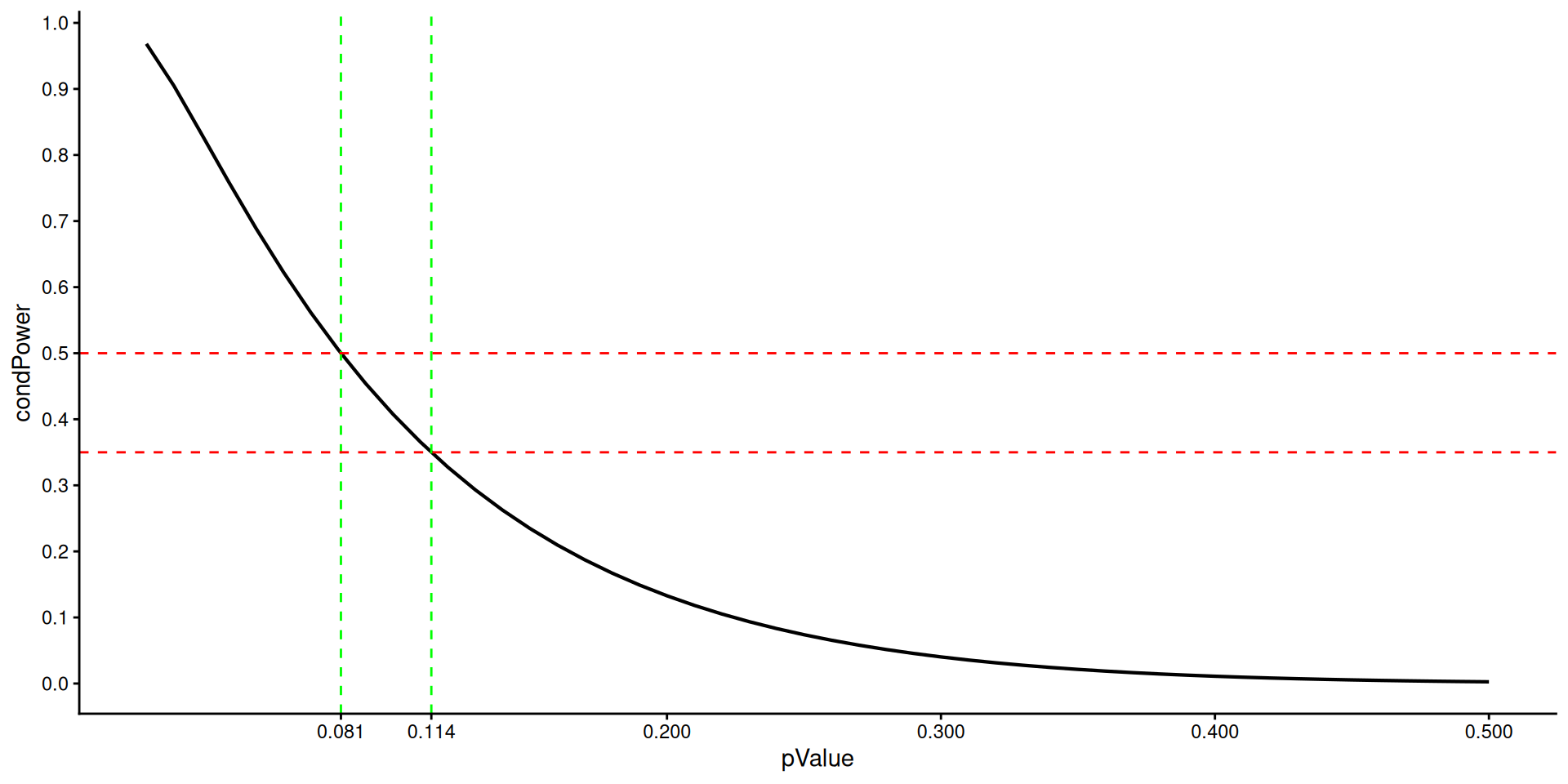
p-value vs. conditional power at observed effect

Promizing zone approach (Mehta and Pocock (2011)): Increase sample size if conditional power at observed effect exceeds 50% (refined values exist). Then traditional test statistic can be used.

design <- getDesignGroupSequential(
    kMax = 2,
    typeOfDesign = "OF",
    alpha = 0.025
)

futilityBounds <- seq(0.01, 0.5, by = 0.01)

y <- design |>
    getFutilityBounds(
        sourceValue = futilityBounds,
        sourceScale = "pValue",
        targetScale = "condPowerAtObserved"
    )

dat <- data.frame(
    pValue = futilityBounds,
    condPower = y
)

ggplot(dat, aes(pValue, condPower)) +
    geom_line(lwd = 0.75) +
    geom_vline(
        xintercept = c(0.081, 0.114),
        linetype = "dashed",
        color = "green",
        lwd = 0.5
    ) +
    geom_hline(
        yintercept = c(0.35, 0.5),
        linetype = "dashed",
        color = "red",
        lwd = 0.5
    ) +
    scale_x_continuous(breaks = c(0.081, 0.114, 0.2, 0.3, 0.4, 0.5)) +
    scale_y_continuous(breaks = seq(0, 1, 0.1)) +
    theme_classic()

p-value vs. conditional power at observed effect

design |>
    getFutilityBounds(
        sourceValue = c(0.35, 0.5),
        sourceScale = "condPowerAtObserved",
        targetScale = "pValue"
    )

[1] 0.11398692 0.08101828

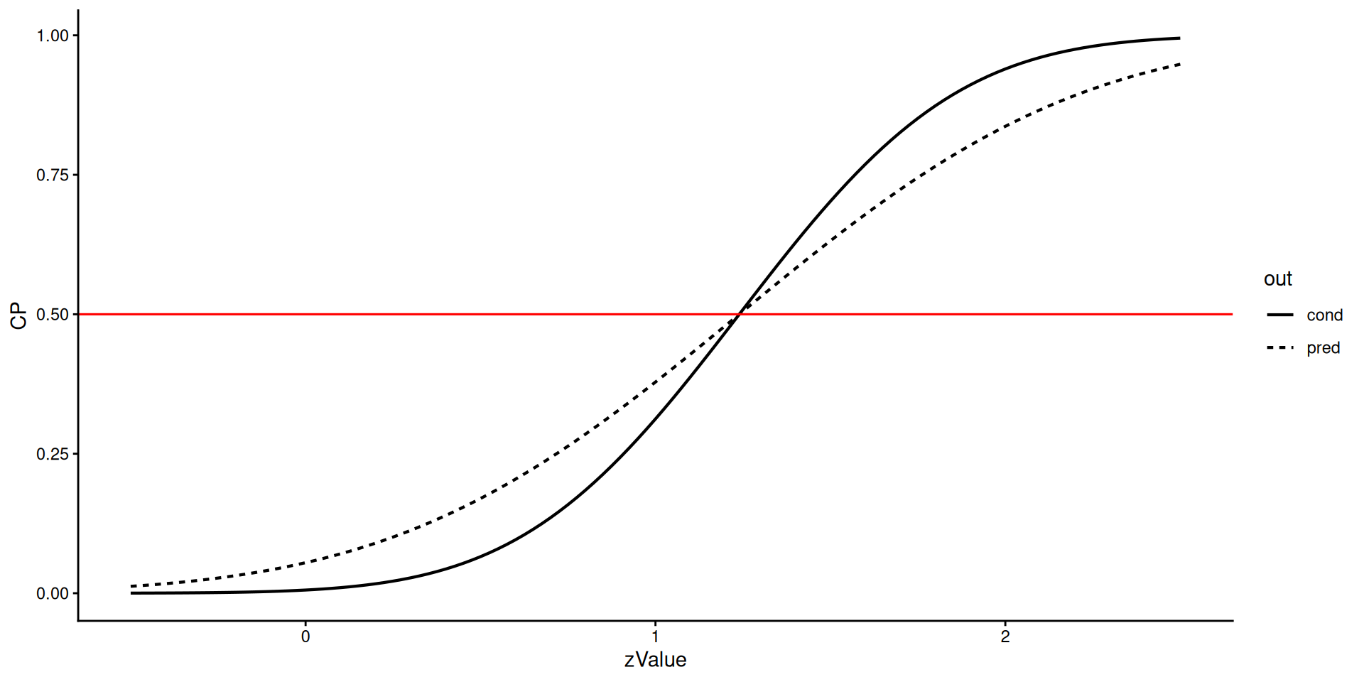
Bayesian predictive power vs. conditional power at observed effect

design <- getDesignGroupSequential(
    typeOfDesign = "noEarlyEfficacy",
    alpha = 0.025,
    informationRates = c(0.4, 1)
)

futilityBounds <- seq(-0.5, 2.5, by = 0.025)

y <- design |>
    getFutilityBounds(
        sourceValue = futilityBounds,
        sourceScale = "zValue",
        targetScale = "predictivePower"
    )
dat <- data.frame(
    zValue = futilityBounds,
    CP = y,
    out = "pred"
)

y <- design |>
    getFutilityBounds(
        sourceValue = futilityBounds,
        sourceScale = "zValue",
        targetScale = "condPowerAtObserved"
    )
dat <- dat |> rbind(
    data.frame(
        zValue = futilityBounds,
        CP = y,
        out = "cond"
    )
)

ggplot(dat, aes(zValue, CP, out)) +
    geom_line(aes(linetype = out), lwd = 0.75) +
    geom_hline(yintercept = 0.5, color = "red", lwd = 0.55) +
    theme_classic()

Bayesian predictive power vs. conditional power at observed effect

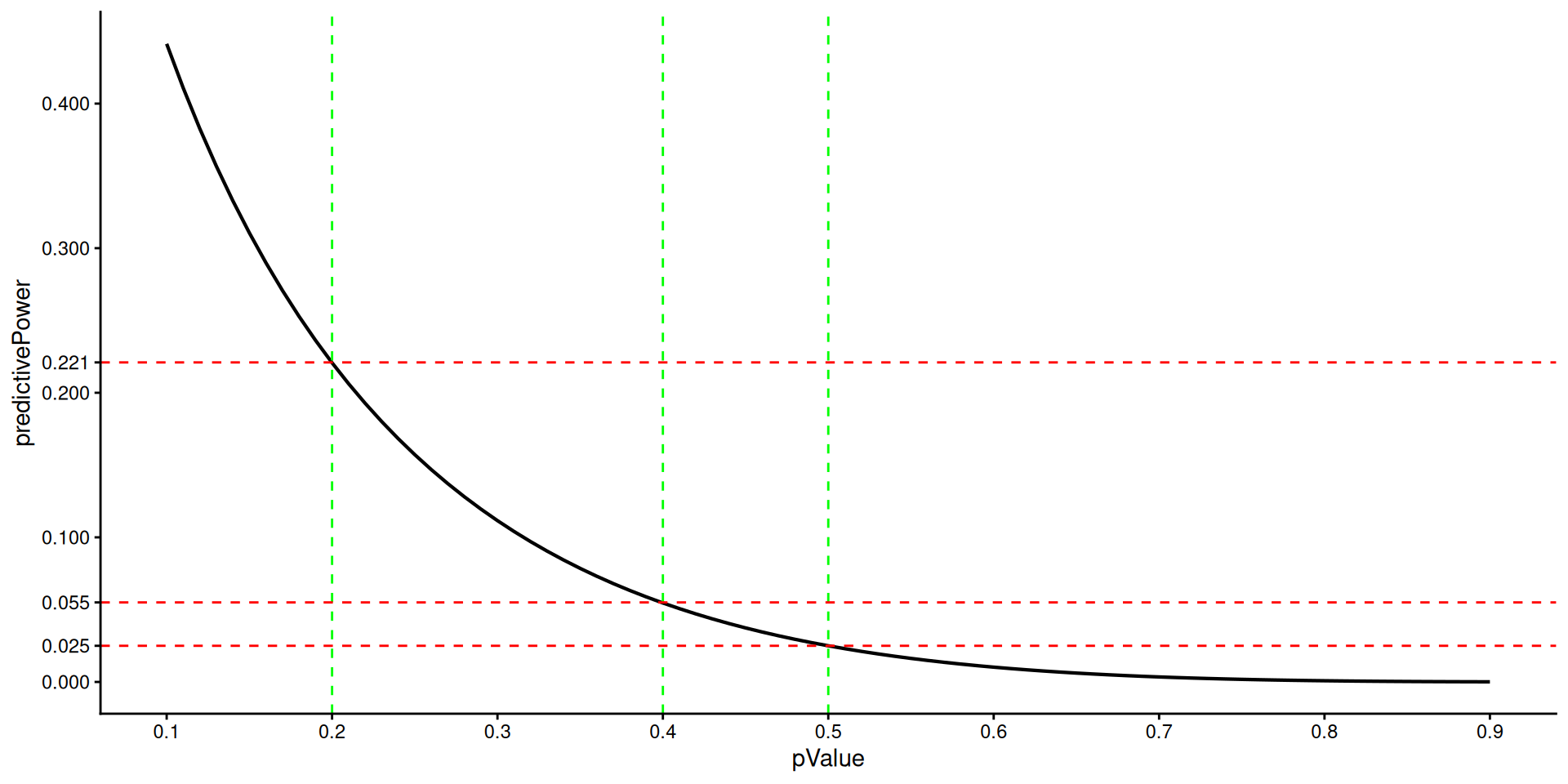
p-value vs. Bayesian predictive power/reverse conditional power

design <- getDesignGroupSequential(
    kMax = 2,
    typeOfDesign = "noEarlyEfficacy",
    alpha = 0.025
)

futilityBounds <- seq(0.1, 0.9, by = 0.01)
y <- design |>
    getFutilityBounds(
        sourceValue = futilityBounds,
        sourceScale = "pValue",
        targetScale = "predictivePower"
    )
dat <- data.frame(
    pValue = futilityBounds,
    predictivePower = y
)

ggplot(dat, aes(pValue, predictivePower)) +
    geom_line(lwd = 0.75) +
    geom_vline(
        xintercept = c(0.2, 0.4, 0.5),
        linetype = "dashed",
        color = "green",
        lwd = 0.5
    ) +
    geom_hline(
        yintercept = c(0.025, 0.055, 0.221),
        linetype = "dashed",
        color = "red",
        lwd = 0.5
    ) +
    scale_x_continuous(breaks = seq(0, 1, 0.1)) +
    scale_y_continuous(breaks = c(0, 0.025, 0.055, 0.1, 0.2, 0.221, 0.3, 0.4)) +
    theme_classic()

p-value vs. Bayesian predictive power/reverse conditional power

design |>
    getFutilityBounds(
        sourceValue = c(0.2, 0.4, 0.5),
        targetScale = "predictivePower",
        sourceScale = "pValue"
        
    )

[1] 0.22072949 0.05461352 0.02500000

Summary

• Several possibilities to define futility stopping
• Predictive interval plots might be another alternative (cf., Ortega-Villa et al. (2025))
• beta spending function might help to construct futility bounds
• All boundaries should be considered as guidelines rather than strict rules, i.e., as a non-binding rule.

• getFutilityBounds() function as a separate tool
• Requires rpact 4.3.0
• Extensively tested, e.g., through reverse checks
• Will be included in sample size and power calculation features, esp., to obtain informations and effect size automatically.

2. Delayed Response

• The delayed response group sequential methodology from Hampson and Jennison (2013) defines a proper consideration of the “pipeline” patients who have been treated at interim but are yet to respond
• getDesignGroupSequential(), getDesignCharacteristics(), and the corresponding getSampleSizexxx() and getPowerxxx() functions characterize a delayed response group sequential test given certain input parameters in terms of power, maximum sample size and expected sample size
• Other approaches can conveniently be handled with the newly published function getGroupSequentialProbabilities()
• Details and examples provided in Vignette Delayed Response Design with rpact.
• Joint work with Stephen Schüürhuis (Schüürhuis, Konietschke, and Kunz (2024) Schüürhuis et al. (2024))

Methodology of Delayed Response Designs

Given boundary sets \(\{u^0_1,\dots,u^0_{K-1}\}\), \(\{u_1,\dots,u_K\}\) and \(\{c_1,\dots,c_K\}\), a \(K\)-stage delayed response group sequential design has the following structure:

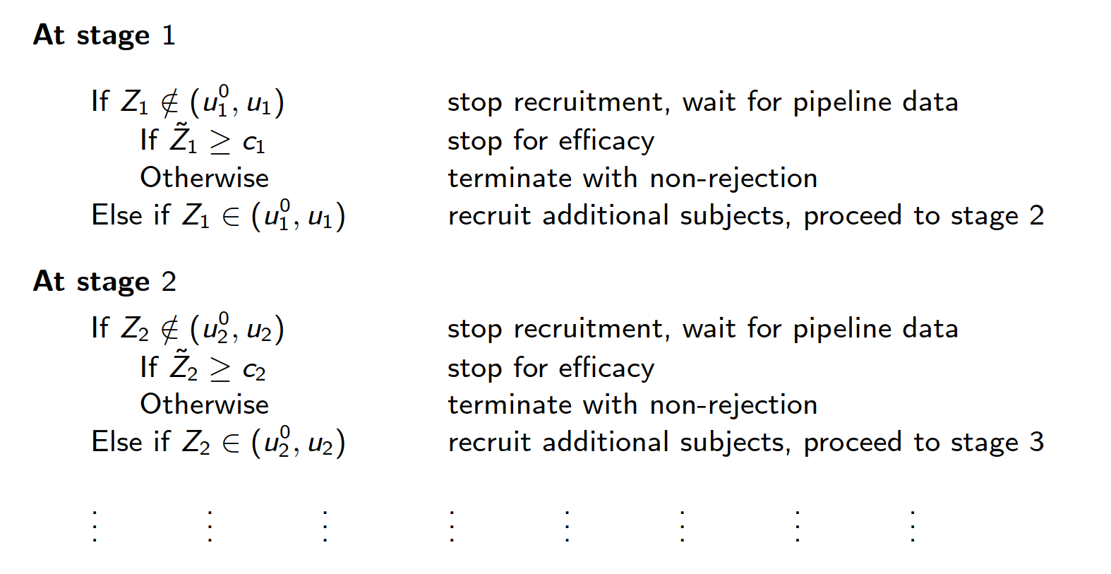
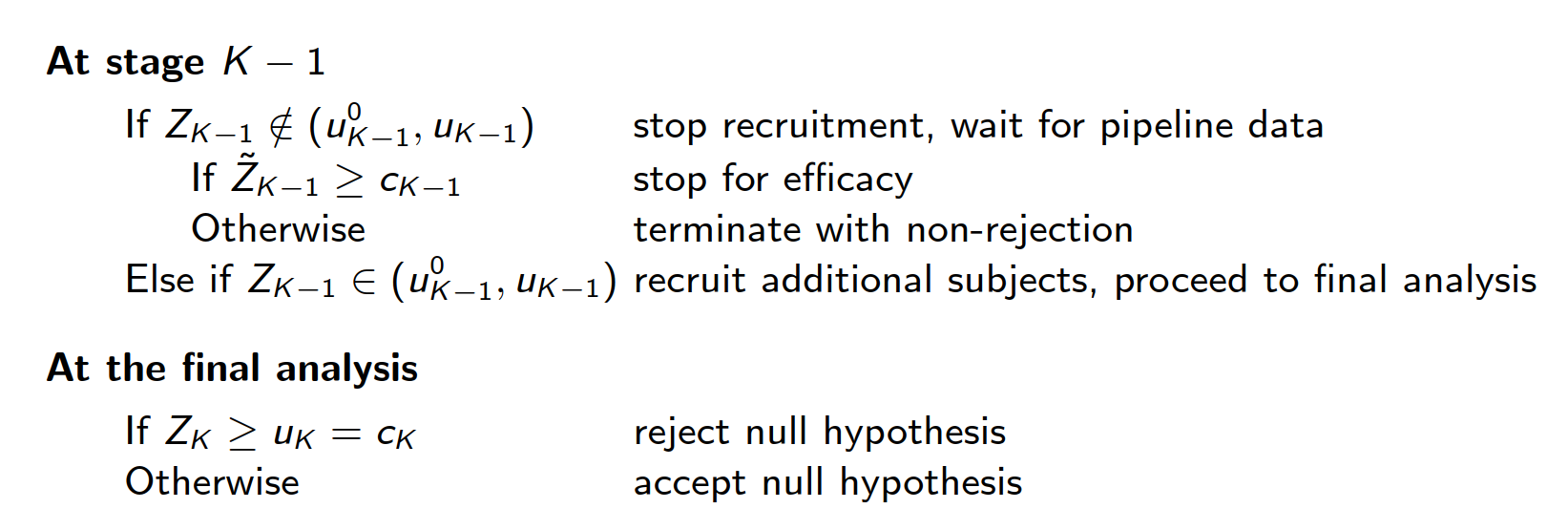
According to Hampson and Jennison (2013), the boundaries \(\{c_1, \dots, c_K\}\) with \(c_K = u_K\) are chosen such that “reversal probabilities” are balanced, to ensure type I error control.

More precisely, \(c_1,\ldots,c_{K - 1}\) are chosen as the (unique) solution of: \[\begin{align*} \begin{split} &P_{H_0}(Z_1 \in (u^0_1, u_1), \dots, Z_{k-1} \in (u^0_{k-1}, u_{k-1}), Z_k \geq u_k, \tilde{Z}_k \leq c_k) \\ &= P_{H_0}(Z_1 \in (u^0_1, u_1), \dots, Z_{k-1} \in (u^0_{k-1}, u_{k-1}), Z_k \leq u^0_k, \tilde{Z}_k \geq c_k). \end{split} \end{align*}\]

Delayed Response: Example

gsdWithDelay <- getDesignGroupSequential(
    kMax = 3,
    alpha = 0.025,
    beta = 0.2,
    typeOfDesign = "asKD",
    gammaA = 2,
    gammaB = 2,
    typeBetaSpending = "bsKD",
    informationRates = c(0.3, 0.7, 1),
    delayedInformation = c(0.16, 0.2),
    bindingFutility = TRUE
)
gsdWithDelay |> summary()

Delayed Response: Example

Sequential analysis with a maximum of 3 looks (delayed response group sequential design)

Kim & DeMets alpha spending design with delayed response (gammaA = 2) and Kim & DeMets beta spending (gammaB = 2), one-sided overall significance level 2.5%, power 80%, undefined endpoint, inflation factor 1.0514, ASN H1 0.9269, ASN H01 0.9329, ASN H0 0.8165.

Stage	1	2	3
Planned information rate	30%	70%	100%
Delayed information	16%	20%
Cumulative alpha spent	0.0022	0.0122	0.0250
Cumulative beta spent	0.0180	0.0980	0.2000
Stage levels (one-sided)	0.0022	0.0109	0.0212
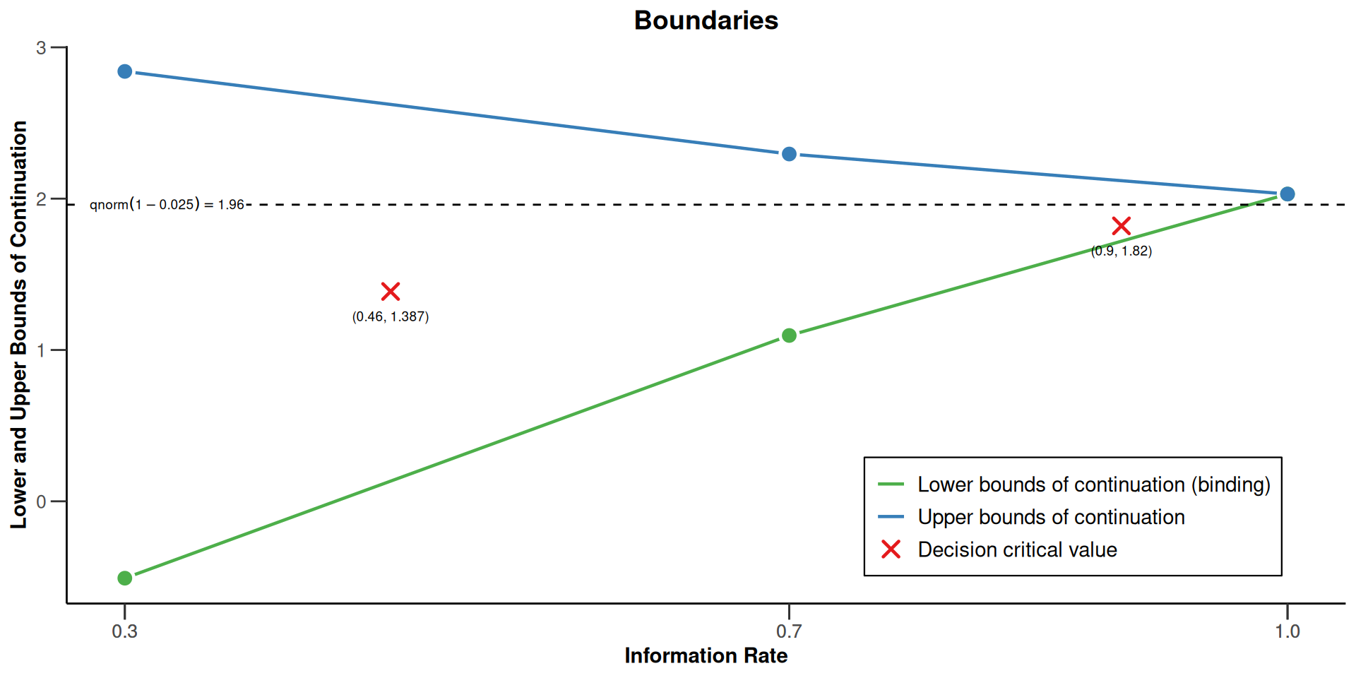
Upper bounds of continuation	2.841	2.295	2.030
Lower bounds of continuation (binding)	-0.508	1.096
Decision critical values	1.387	1.820	2.030
Reversal probabilities	<0.0001	0.0018
Cumulative power	0.1026	0.5563	0.8000
Futility probabilities under H1	0.019	0.083

Delayed Response: Plot

gsdWithDelay |> plot()

3. Count Data

• getSampleSizeCounts() and getPowerCounts()
  • Perform sample size calculations and the assessment of test characteristics for clinical trials with negative binomial distributed count data.
  • Fixed sample size and group sequential designs (Mütze et al. (2019))
  • Perform blinded sample size reassessments according to Friede and Schmidli (2010)
  • Output boundary values also on the treatment effect scale
• New function getSimulationCounts()
  • Perform power simulations for clinical trials with negative binomial distributed count data
  • Simulated power, stopping probabilities, conditional power, and expected sample size for testing mean rates for negative binomial distributed event numbers in the two treatment groups testing situation

Count Data: Options

• Either both event rates \(\lambda_1\) and \(\lambda_2\), or \(\lambda_2\) and rate ratio \(\theta\), or \(\lambda\) and \(\theta\) (blinded sample size reassessment!)
• \(\lambda_1\) and \(\theta\) can be vectors
• Different ways of calculation:
  • fixed exposure time,
  • accrual and study time,
  • or accrual and fixed number of patients
• Staggered patient entry
• Group sequential or fixed sample size setting
• Details and examples provided in Vignette Count Data with rpact

Count Data: Simple Example

getSampleSizeCounts(
    alpha = 0.05,
    beta = 0.1,
    sided = 2,
    lambda2 = 0.4,
    theta = 0.75,
    overdispersion = 0.5,
    fixedExposureTime = 1
) |> summary()

Count Data: Simple Example

Sample size calculation for a count data endpoint

Fixed sample analysis, two-sided significance level 5%, power 90%. The results were calculated for a two-sample Wald-test for count data, H0: lambda(1) / lambda(2) = 1, H1: effect = 0.75, lambda(2) = 0.4, overdispersion = 0.5, fixed exposure time = 1.

Stage	Fixed
Stage level (two-sided)	0.0500
Efficacy boundary (z-value scale)	1.960
Lower efficacy boundary (t)	0.844
Upper efficacy boundary (t)	1.171
Lambda(1)	0.300
Number of subjects	1736.0
Maximum information	127.0

Legend:

• (t): treatment effect scale

Count Data: Power Calculation

getPowerCounts(
    directionUpper = FALSE,
    lambda2 = 1.4,
    theta = c(0.75, 1),
    overdispersion = 0.7,
    maxNumberOfSubjects = 300,
    followUpTime = 12,
    accrualTime = 12
) |> fetch(overallReject)

$overallReject
[1] 0.8213803 0.0250000

Count Data: Power Simulation

tictoc::tic()
getSimulationCounts(
    directionUpper = FALSE,
    lambda2 = 1.4,
    theta = c(0.75, 1),
    overdispersion = 0.7,
    maxNumberOfSubjects = 300,
    plannedCalendarTime = 24,
    accrualTime = 12,
    fixedExposureTime = 12,
    # followUpTime = 12,
    maxNumberOfIterations = 1000,
    seed = 123
) |> fetch(overallReject)

$overallReject
[1] 0.835 0.028

tictoc::toc()

1.308 sec elapsed

RPACT Cloud

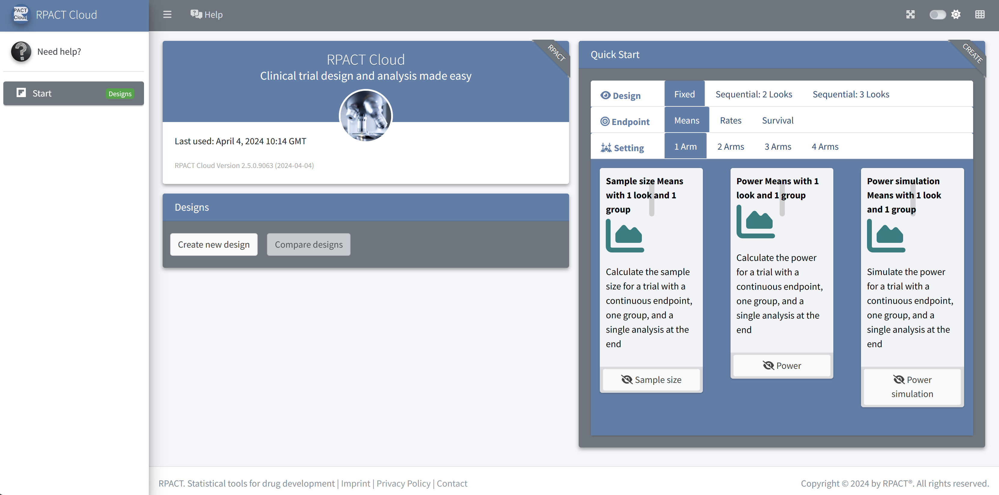
RPACT Cloud ☁️

• Graphical user interface

• Web based usage without local installation on nearly any device

• Provides an easy entry to to learn and demonstrate the usage of rpact

• Starting point for your R Markdown or Quarto reports

• Online available at rpact.cloud

Start Page

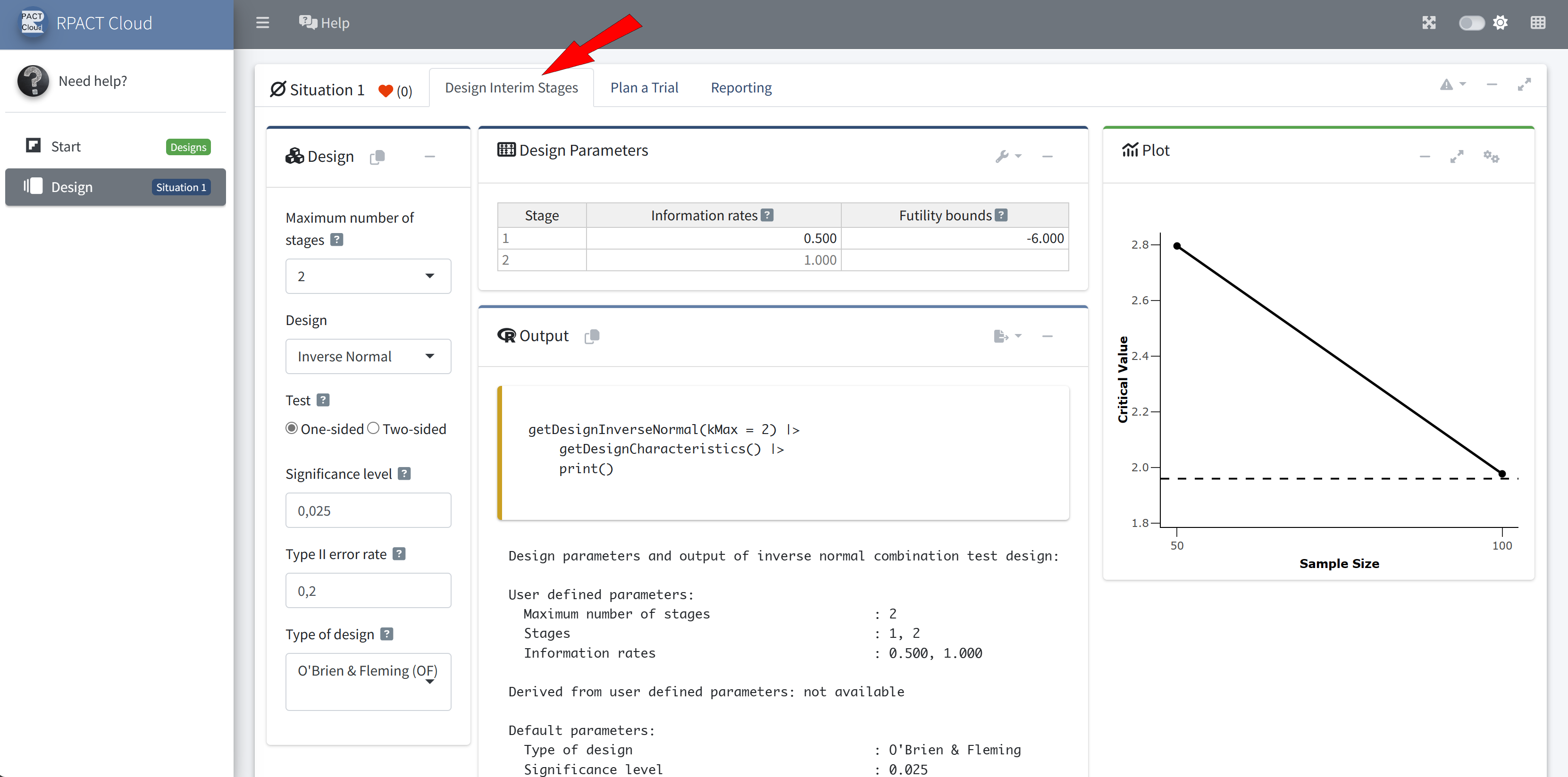
Design

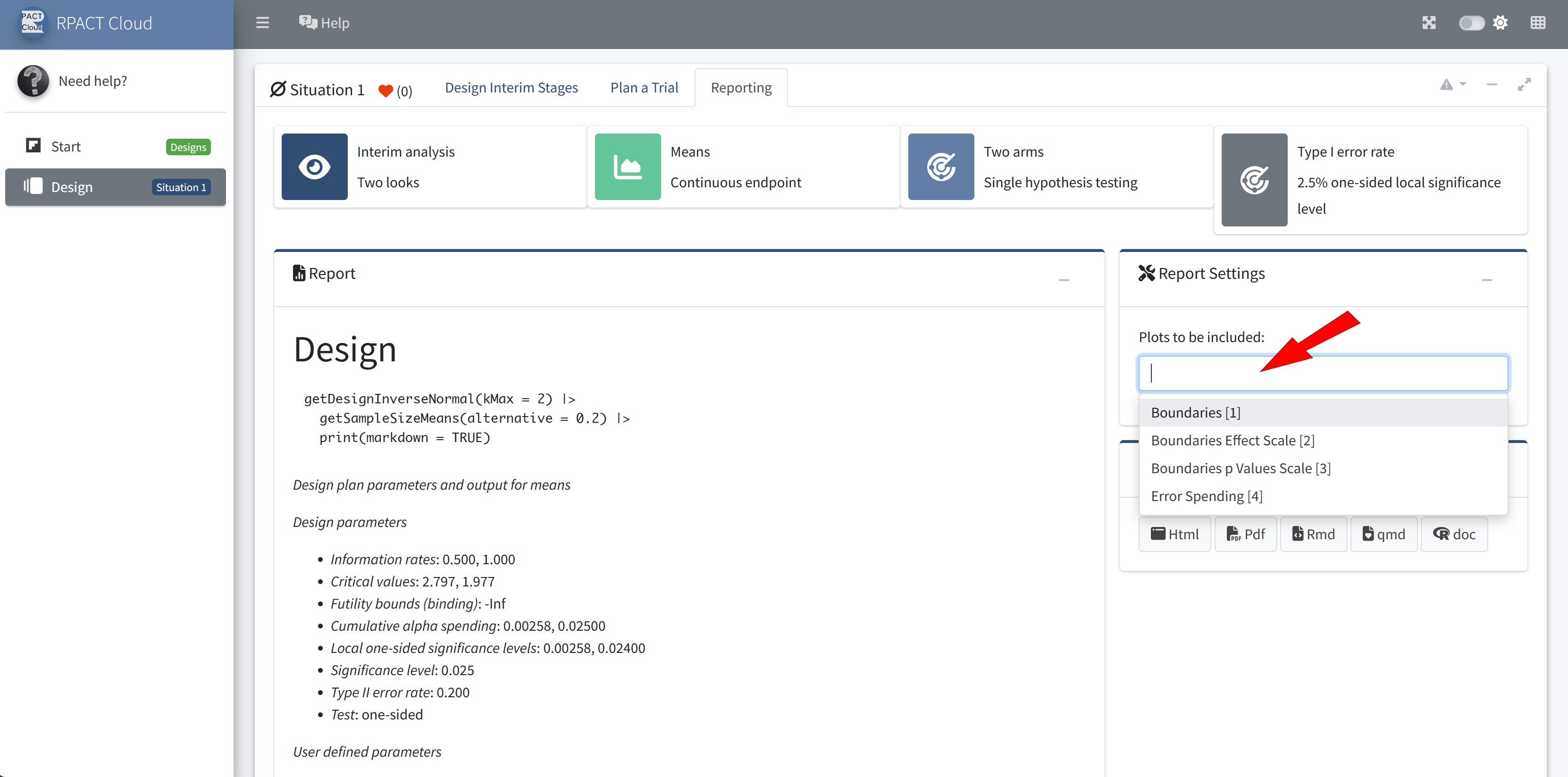
Reporting

What’s Next?

New Package Features

Just in the near future you will see in rpact:

• Patient level survival data simulations for multi-arm and enrichment designs
• Optimum conditional error functions according to Brannath et al. (2024) (package optconerrf published on CRAN Sep 09, 2025)
• Least square means interface for continuous endpoints

The R Package rpact - Online Resources

Further information, installation, and usage:

• CRAN: cran.r-project.org/package=rpact
• GitHub: github.com/rpact-com/rpact
• GitHub Pages: rpact-com.github.io/rpact
• OpenSci R-universe: rpact-com.r-universe.dev/rpact
• METACRAN: r-pkg.org/pkg/rpact
• Codecov: app.codecov.io/gh/rpact-com/rpact
• RPACT manual and vignettes: rpact.org
• RPACT validation and training: rpact.com

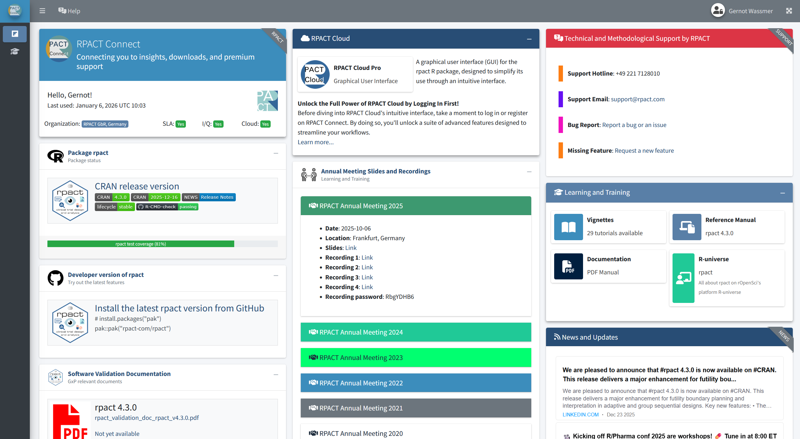
All information and resources about RPACT on one dashboard page

RPACT Connect: connect.rpact.com

RPACT Connect

Thank you!

References

Brannath, W., M. Dreher, J. Verth, and M. Scharpenberg. 2024. “Optimal Monotone Conditional Error Functions.” arXiv Preprint arXiv:2402.00814.

Friede, Tim, and Heinz Schmidli. 2010. “Blinded Sample Size Reestimation with Count Data: Methods and Applications in Multiple Sclerosis.” Statistics in Medicine 29 (10): 1145–56.

Hampson, Lisa V., and Christopher Jennison. 2013. “Group Sequential Tests for Delayed Responses (with Discussion).” Journal of the Royal Statistical Society Series B: Statistical Methodology 75 (1): 3–54. https://doi.org/10.1111/j.1467-9868.2012.01030.x.

Mehta, Cyrus R, and Stuart J Pocock. 2011. “Adaptive Increase in Sample Size When Interim Results Are Promising: A Practical Guide with Examples.” Statistics in Medicine 30 (28): 3267–84.

Mütze, Tobias, Ekkehard Glimm, Heinz Schmidli, and Tim Friede. 2019. “Group Sequential Designs for Negative Binomial Outcomes.” Statistical Methods in Medical Research 28 (8): 2326–47. https://doi.org/10.1177/0962280218773115.

Ortega-Villa, Ana M, Megan C Grieco, Kevin Rubenstein, Jing Wang, and Michael A Proschan. 2025. “Futility Monitoring in Clinical Trials.” Statistics in Medicine 44 (13-14): e70157.

Robertson, D. S., Thomas Burnett, Babak Choodari-Oskooei, Munya Dimairo, Michael Grayling, Philip Pallmann, and Thomas Jaki. 2025. “Confidence Intervals for Adaptive Trial Designs I: A Methodological Review.” Statistics in Medicine 44 (18-19): e70174.

Robertson, D. S., Babak Choodari-Oskooei, Munya Dimairo, Laura Flight, Philip Pallmann, and Thomas Jaki. 2023. “Point Estimation for Adaptive Trial Designs I: A Methodological Review.” Statistics in Medicine 42 (2): 122–45.

Schüürhuis, Stephen, Frank Konietschke, and Cornelia Ursula Kunz. 2024. “A Two-Stage Group-Sequential Design for Delayed Treatment Responses with the Possibility of Trial Restart.” Statistics in Medicine 43: 2368–88.

Schüürhuis, Stephen, Gernot Wassmer, Friedrich Pahlke, Meinhard Kieser, Frank Konietschke, and Carolin Herrmann. 2024. “Two-Stage Group-Sequential Designs with Delayed Responses – What Is the Point of Applying Corresponding Methods?” BMC Medical Research Methodology 24: 242.

Tan, Ming, Xiaoping Xiong, and Michael H Kutner. 1998. “Clinical Trial Designs Based on Sequential Conditional Probability Ratio Tests and Reverse Stochastic Curtailing.” Biometrics, 682–95.

Wassmer, Gernot, and Werner Brannath. 2016. Group Sequential and Confirmatory Adaptive Designs in Clinical Trials. Springer.

———. 2025. Group Sequential and Confirmatory Adaptive Designs in Clinical Trials. 2nd ed. Springer. https://link.springer.com/book/10.1007/978-3-031-89669-9.